Chapter 2: Genetic Causes of Behavior
Barry Sinervo
Table of Contents
Introduction
to Genetic Terms and Mendelian Traits
The Genotype
and Phenotype
Side
Box 2.1: Mutation, Segregation, and Recombination
Mutation
Segregation
Recombination
Components
of Phenotypic and Genetic Variation
Side Box 2.2: Additive Genetic Variation versus Dominance
Variation
Co-dominant
alleles
Dominant
and recessive alleles
Overdominance
Underdominance
Mendelian
Traits
Behavioral
Mutants in the Laboratory: Roving versus Sitting in Drosophila larvae
Beak Size and Seed Preference in African Finches
Side Box
2.4: Random Mating and Hardy-Weinberg Gene Frequencies
Random
Mating Finches
Mendelian Inheritance of Three Alleles
Molecular
Tools of Behavioral Geneticists
Mutation
Analysis of a Gene for Parental Care in Mice: fosB
Paternity Analysis and a Gene for Alternative Male
Strategy in the Ruff
Epistatic Genes for Alternative Male Strategy and
Sex Transformation in Marine Isopods
Polygenic
Inheritance
Heritability
of IQ
Side Box
2.5: Heritability
Side Box
2.6: Additive versus Dominance Variation
Environmental
Effects on Phenotype
Condition-dependent
strategies and alternative male types
Alternative Larval Types in Spadefoot Toads and Tiger
Salamanders
Study
Questions for Chapter 2
When we search for the proximate
factors for behavioral causes, we naturally start with genes. When the fusion
of sperm and egg produces a zygote, the stage is set for a cascade of developmental
events that lead to the production of the phenotype. The central dogma of biology
holds that DNA from alleles at a genetic locus translates into proteins. Structural
proteins are used to contract the cells, and enzymatic proteins provide the
basis for cellular machinery. Cells in the developing zygote interact mechanically
or chemically with adjacent cells, or cells can produce "messengers" that facilitate
the cell-cell interaction at distance. Cell-cell and organ-mediated interactions
cause a cascade of events that we collectively refer to as development. The
embryo is gradually organized into a functioning animal with nerves and organ
systems that begin to regulate behaviors. Those behaviors have functional or
selective consequences. Individuals selectively live, breed and die according
to their phenotype. Gene frequencies change across the generation and the species
evolves.
The goal for this chapter is
to develop an understanding of the genetic factors that govern the expression
of morphological traits associated with alternative behaviors. Techniques of
classical genetics such as genetic crosses and pedigree analyses are now being
combined with tools of molecular biology to identify specific genes that appear
to govern the expression of complex behaviors. Before we begin this quest, let
us arm ourselves with a few of the terms of genetics (distilled from Keller
and Lloyd, 1992). In particular, we focus on those genetic processes that deal
with genetic variation within and among individuals.
The
Genotype and Phenotype
- Genotype --
the sum total of all the alleles at all the loci in a organism. While precise
and concise, this definition is not very useful. The genotype may also apply
to genetic material at a single genetic locus and describe the alleles that
an individual possesses at a particular locus. The two alleles at a genetic
locus come from the male and female parents and form the basic unit of genetic
variation in an individual. The process of meiosis, mendelian segregation,
and recombination among all the myriad of genetic loci in an individual effectively
makes each sexually-produced individual unique (see Side Box 2.1. Mutation,
Segregation and Recombination). In contrast, an asexual organism is a genetic
clone of its female parent. The genotype is largely static for an individual
during its lifetime, except when a mutation occurs. A mutation is a
lesion of DNA that changes the genetic material in one allele at a locus.
If the mutation occurs in a somatic cell, there will be no consequence for
transmission of material across generations. However, if the mutation occurs
in a cell of the germ line, which produces sperm or eggs for sexual reproduction,
then the mutation can be transmitted across generations. Mutations are the
ultimate source of all genetic variation.
Phenotype -- the
external expression of the genes, and the result of a gene's interaction with
the environment. This includes mechanisms of development. Because the stage
of development depends on age, the phenotype can be highly labile,
or can change dramatically during its lifetime. The organism develops, it
learns, it acclimates and its phenotype changes accordingly. For simplicity
of analysis, we break the whole organism into phenotypic traits that
are largely functional units. For example, the number of offspring that an
animal produces in one bout of reproduction, termed fecundity, is a phenotypic
trait related to reproduction. Likewise, the kind of parental care is a second
phenotypic trait related to reproduction. However, phenotypic traits are usually
correlated with other phenotypic traits and such correlations arise
from proximate mechanism. For example, the number of offspring that a parent
produces is related to the kind or quality of care that the parent can provide
to the offspring. Usually we refer to such relationships as fitness trade-offs
because an increase in one fitness trait (fecundity) has an impact on a correlated
trait (quality of care). The proximate mechanisms that link these particular
traits are related to energy and metabolism. Rearing large numbers of offspring
requires more total energy to keep the level of care constant for each offspring.
Alternatively, less energy (or lower quality care) is available for each offspring.
Environment -- the
environment is anything external to the genetic material. For example, food
availability in part determines body weight. In animals that lay eggs without
parental care, the eggs are subjected to environmental variation in the form
of temperature, hydration, or perhaps salinity. In animals which lay eggs
and have extended parental care in a nest, the environment is a function of
the parents and perhaps the other sib-mates in the nest. In animals with internal
fertilization and some kind of gestation, the mother's physiology per se becomes
an important component of the offspring's environment. Regardless of whether
or not an organism requires extended parental care as a juvenile, the environment
still plays a major role in that individual's development. Of course, there
is a second sense in which the environment interacts with the genotype and
phenotype: the environment causes natural selection. While this natural selection
acts on phenotypes within a generation (e.g., the parents, its effects are
transmitted to the next generation (e.g., offspring). -
A simple expression describes
the relationship between the variation in a particular phenotypic trait among
individuals found in a single population:
where
P, G, and E are phenotypic, genotypic, and environmental
variation in the trait. If the environmental variation is large, then little
phenotypic variation arises due to genetic sources of variation. Conversely,
if genetic variation is large, then the phenotypic trait is largely determined
by genetic factors. As we have seen, heritable or genetic variation is central
to Darwin’s theory of natural selection, and evolutionary change will occur
more rapidly for traits that are strongly determined by genetic factors.
The process of natural selection
is often characterized as "blind" and this is largely because the source of
all genetic variation is largely a stochastic process. The ultimate source of
genetic variation is mutations; however, segregation, and recombination provide
an stochastic mechanisms for randomizing genetic variation in a population.
While mutations alter DNA by changing base pairs, segregation and recombination
do not alter the material content of DNA. Instead they provide powerful mechanisms
for mixing up the DNA during sexual reproduction.
Mutation
The process of mutation is probabilistic.
We describe the process in terms of the probability of a mutation occurring
in an individual during its lifetime. Typical rates of mutation are between
1 in 10,000 (10-4) and 1 in 1,000,000 (10-6)
for many organisms. Either this means that a long time must pass before a mutation
occurs in a population, or the population must be very large. The population
must number in excess of 106 or one million members
in order to see an average of one mutation per generation for a gene with a
mutation rate of 10-6. Most mutations are detrimental,
and perhaps only 1 in 1,000 is beneficial. Thus, in this population of a million
we might have to wait for one thousand years for a specific genetic locus to
throw us a beneficial mutation (of course there are thousands of possible loci
in an organism so the waiting time for any beneficial mutation is less). Even
if a mutation arises, there is no guarantee that natural selection will act
on it.
We
can calculate the probability that a beneficial mutation makes it through meiosis
and segregation. A beneficial mutation occurs within a diploid parent which
has two copies of each gene. The beneficial mutation has a 50% chance of being
transmitted to any one offspring and a 50% chance of not being passed on. With
an organism that has four progeny, the probability of a single offspring not
getting the beneficial mutation is independent of the other offspring
not getting the mutant allele. By using the laws of probability we can multiply
successive independent events to compute the probability that none of the four
progeny gets the beneficial mutation:
1/2 x 1/2 x 1/2 x 1/2 = 1/16.
If the unique beneficial mutation
is not passed on to the progeny, then more time will be required for a new beneficial
mutation to arise in the population. At this point, natural selection has a
chance of promoting its spread through the population.
Segregation
Genes are found on chromosomes.
The first random event in sexual reproduction occurs during meiosis when homologous
pairs of chromosomes line up on the equatorial plate in preparation for the
cell division that reduces a diploid (2N) cell of the germ line to an haploid
(N) gamete. During the process of segregation different homologues will randomly
be distributed between the two daughter chromosomes, gametes end up with very
different chromosome complements. Given that the total number of chromosomes
is C, then there are 2 raised to the power of C different gametes that could
be produced from segregation of chromosomes (in humans that would be 246).
Segregation can produce a vast number of different gametes and is a potent mixer
of variation in sexual organisms.
Recombination
Recombination
between homologous pairs of chromosomes during meiosis can generate even more
gamete types. The chromosome is loaded with recombinational hotspots. Any given
chromosome will typically recombine with its homologue at one or two points
during a given meiotic event (recombination rate on a given chromosome is a
function of chromosome length). However, the recombination points for two different
meiotic events can be different. Given that gametes such as sperm are generated
by millions of different meiotic events, the number of potential gamete types
from a single parent is vast. If one considers all possible parents in a modest-sized
breeding population such as humans (5 billion), there are easily more potential
recombination products than molecules in the known universe.
<END SIDE BOX>
Components
of Phenotypic and Genetic Variation
We can follow a roadmap from
genotype to phenotype, but the route is rarely a one to one mapping between
genes and phenotypic traits. Environment further obscures the relationship between
genotype and phenotype. We have several hierarchical concepts that describe
how genotype can be related to phenotypic traits. These additional terms describe
different levels of genetic interaction and their effect on genotype and phenotype:
- the effect of one allele on another
allele at the same genetic locus (e.g., additive effect versus dominance),
- the effect of one genetic locus
on another independent locus (e.g., polygenic and epistasis),
- the effect of a single gene or
two or more phenotypic traits (e.g., pleiotropy),
- the effect of two or more genes
on a single phenotypic trait (e.g., additive, epistasis),
- the interaction between genetic
factors and the environment (e.g, norm of reaction).
Pleiotropy -- a
single gene that has an effect on the expression of two or more phenotypic
traits is said to have a pleiotropic effect on the traits. For example, testosterone
controls the development of what are referred to as secondary sexual characteristics
(e.g., a lion's mane), but testosterone also relates to behavioral traits
like aggression. Thus, a gene that controls the levels of testosterone would
have a pleiotropic effect on the expression of many secondary sexual traits
which are morphological, as well as behavioral. The concept of pleiotropy
is intimately related to the concept of trade-off (Stearns 1976). Pleiotropy
describes the proximate genetic source for many phenotypic trade-offs. If
one gene controls the expression of two or more traits and those traits are
related to a fitness trade-off, then we have identified the proximate source
of the trade-off.
Polygenic -- if
two or more genes are responsible for a single trait, the phenotypic trait
is said to be governed by polygenic factors. For example, growth rate is undoubtedly
caused by a number of genes that act in a complex cascade. Body size, which
is the result of a large number of genes, is polygenically determined. Genes
that control growth hormone have a large effect on body size. Likewise, genes
that control sex steroids like testosterone have some effect on body size,
especially during maturation phases of growth. Undoubtedly, many genes that
influence metabolism have a small, but measurable effect on body size.
Additive effects within and between loci. The
simplest additive genetic relationship occurs between two alleles at the same
genetic locus. If two alleles are co-dominant, then the heterozygote is exactly
intermediate in phenotype relative to the two homozygous types. In this idealized
case, "the effect of substituting one allele for another is additive in its
effect on phenotype". Just like alleles acting in an additive fashion at a
single locus, polygenic genetic loci can also interact in an additive fashion
to produce a phenotype. If two or more genes have a simple effect on the phenotype
they are generally thought of as having an additive effect. If a trait results
from two or more genes then an additive relationship between them would lead
to the simplest kind of polygenic inheritance. Additive genetic variance
is what underlies the notion of heritability and is responsible for the similarity
between parents and offspring. Natural selection operates on additive genetic
variation because additive genetic variation is largely responsible for the
resemblance or heritability between parents and offspring (see Side Box 2.2:
Additive Genetic versus Dominance Variation).
Dominance. Interactions
between alleles at a single locus are termed dominance interactions.
For example, if an allele is said to be recessive to another allele, then
an individual that possesses a copy of the dominant allele and a
copy of the recessive allele (e.g., heterozygote) will be
phenotypically identical to an individual that possesses two copies of the
dominant allele (e.g., homozygous). The "recessive phenotype"
is only expressed if the individual is homozygous for two of the recessive
alleles. The rover and sitter gene of Drosophila larvae discussed
below is a classic example of the effect of a dominant gene on behavior.
If two genes are co-dominant then the heterozygote is intermediate between
the two homozygous genotypes and the alleles are additive in their effect.
While dominance variation can be a very large component of the total genetic
variation of a phenotypic trait, dominance variation is entirely non-additive
(see Side Box 2.2).
Epistasis. If
two different genetic loci interact in any way that is not additive,
then they are said to act epistatically. Many pigmentation genes act in an
epistatic fashion. The simplest example of epistasis relates to genes that
control pigmentation. This example illustrates how a HREF=#anchor214836 between
alleles at the same locus is conceptually similar to an epistatic interaction
between two genetic loci. Consider a single locus such as the coat color of
a popular breed of dog the Labrador Retriever. The color yellow (y) is recessive
to black (b). One copy of the black allele and production of the black pigment
overwhelms the expression of the yellow coated phenotype and a heterozygous
yb individual is black. The effect of the black pigment is non-additive, in
that one copy completely masks the recessive yellow. A second coat color locus
codes for production of brown pigment. The brown locus interacts in a non-additive
fashion in that an individual with an allele at the brown locus can be brown
regardless what pigment is expressed at the black locus. The brown locus overwhelms
the expression of the black locus in a non-additive fashion, but in this case,
brown interacts epistatically with the black locus.
Genotype and Environment Interaction and Phenotypic
plasticity. If the expression
of a gene depends on the environment in any way, then the phenotype is said
to be due to an interaction between the genotype and environment. This idea
is central to behavior and we will explore it in great detail in upcoming
chapters. For example, birds undoubtedly have genes for learning, and indeed
some species of birds may differ in how they learn. A famous example of genotype
environment interactions relates to how birds learned to open milk bottles
in England. For years milkman in England left milk bottles outside on the
porch with no problems. One day a single bird learned how to open the top
of the milk bottles and drink the milk. This trait was passed on to other
birds by learning. Even different species of birds learned the task. Here
the environment changed, with the advent of a single bird learning to opening
milk bottles. However, only some species of birds learned how to open milk
bottles, other species did not. Learning was presumably contingent on both
the environment and on the genes for learning in each species. Both the presence
and absence of milk bottles, and presence or absence of a tutor bird to teach
naive birds was necessary for learning this task.
Phenotypic plasticity -- the
expression of different alternative phenotypes within a constant genetic background.
While, there are few genetic differences among individuals some environmental
cue (predictable) causes development to proceed along different pathways.
From a single genotype, many different phenotypes can be produced. -
What is the source of heritable variation? The
resemblance between parents and offspring is entirely due to the additive effect
that genes have on phenotype. Not all genetic variation is additive. For example,
dominance variation arises from the degree to which one allele at a locus alters
the effect of the allele on the complementary chromosome. A useful way to think
about additive genetic variation is to consider the proportion of the phenotype
that can be predicted from a knowledge of the number of A versus a
alleles that are present in the genotype -- or the genotypic value. Consider
an aa individual to have zero A alleles, Aa has one A
allele, and AA has two A alleles. Only in the idealized case when
alleles at a genetic locus are co-dominant, are the genes said to act in a purely
additive fashion. Dominance reduces the additive genetic variation, increasing
the dominance variation at the same time.
|

|
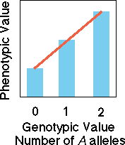
Co-dominant
alleles
In the case of a co-dominant
set of alleles, knowledge of genotype allows us to perfectly predict the
value of the phenotype. A regression (red line) of phenotypic value on
the number of A alleles or the genotypic value yields a perfect
predictive line.
|
|

|
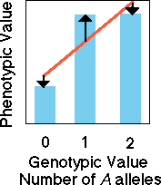
Dominant
and recessive alleles
In the case of a dominant
A allele, knowledge of genotypic value allows us to only imperfectly
predict the value of the phenotype. Because heterozygotes and dominant
homozygotes have the same phenotypic value, the fit between the regression
(red line) of phenotypic value on genotypic value has error (black arrows).
There is still a significant regression slope showing that some of the
variation is due to additive genetic causes (red line) and some is due
to dominance variation (black arrows).
|
|

|
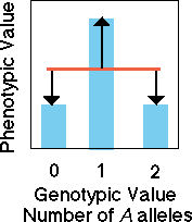
Overdominance
In the case of overdominance,
knowledge of genotype does not allow us to confidently predict the value
of the phenotype. There is no slope to the regression line so none of
the variation is due to "additive genetic effects" of alleles. All variation
in our model is due to error in our model which arises from dominance
variation (black arrows). Consider two parents that are homozygous for
alternative alleles (aa and AA). If behavior were strongly
determined by an overdominant allele then the heterozygous progeny would
not at all resemble the homozygous parents.
|
|

|
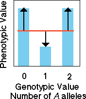
Underdominance
Likewise, in the case of underdominance,
knowledge of genotype does not allow us to predict the value of the phenotype
with any confidence. There is no slope to the regression line so none
of the variation is due to "additive genetic effects" of alleles. All
variation in our model is due to error in our model which arises from
dominance variation (black arrows).
|
<END SIDE BOX>
We will explore many of these
issues of genetics through examples. I have chosen a diverse set of behavioral
traits to introduce many concepts in animal behavior which will be covered in
greater detail in later chapters. Each example, illustrates one of the genetic
terms discussed above. In many cases model organisms studied in the laboratory
facilitate our study of behavioral causes because of the large sample sizes
possible in the laboratory allow for necessary statistical power required to
assess genetic bases of behavioral traits. Other genetic examples are drawn
from natural populations. While it is more difficult to collect genetic data
on animals in the wild, these larger animals provide answers to natural selection
because we can follow them through their lives. Moreover, it is essential to
study animals in the wild so that we can infer how their actions are reflected
in the process of natural or sexual selection. By long-term observation of animals
in the wild, we are able to reconstruct present day patterns of selection (Lande,
1983) that may have been historically significant during the origin of behavioral
traits. A first step in selection analyses is determining the genetic basis
of behavioral traits. Classic genetic crosses and pedigree analyses are the
standard tools of a behavioral geneticist.
Behavioral
Mutants in the Laboratory: Roving versus Sitting in Drosophila larvae
Many of the basic issues of
mendelian inheritance of animal behavior are found in the example of roving
versus sitting larvae in Drosophila. Marie Sokolowski and her colleagues
(Sokolowski 1985; de Belle and Sokolowski 1987) generated two strains of larvae
and then carried out some illuminating crosses. If you cross parental rover
males and sitter females, each of the ensuing strains is pure and homozygous
for either the rover or sitter allele. Crossing two pure parental lines (P0)
produces progeny which are referred to as the F1. In theory, if the phenotype
rests entirely on a single gene with two alternative alleles (a dominant rover
allele and a recessive sitter allele). The F1 cross produces all rovers with
no sitters. In practice, this cross produces nearly all rovers, suggesting that
sitter is recessive to rover (or rover is dominant to sitter). The telling bit
of evidence arises from a cross between F1 progeny, which should produce 3 genotypes
(see Punnett Square in Table 2.1.A), but only two phenotypes (see Table 2.1.B),
owing to dominance of the R allele over the S allele. These offspring produce
rovers and sitters in nearly a 3:1 ratio -- exactly the pattern one expects
if the F1 are all heterozygous for rover and sitter alleles.
|
Table 2.1. A) Theoretical Results from F1 X F1 cross
|
genotype of first parent
|
|
Table 2.1.B) Observed Phenotype in F2.
|
Hypothesized genotype
|
Predicted Ratio
|
|
|
R
|
S
|
|
Rover
|
R|R
|
1
|
|
genotye of
|
R
|
R|R
|
R|S
|
|
Rover
|
R|S
|
2
|
|
second parent
|
S
|
R|S
|
S|S
|
|
Sitter
|
S|S
|
1
|
Beak
Size and Seed Preference in African Finches
Like the behavioral morphs of
fruitflies, species of African Finch that inhabits Cameroon, Pyrenestes ostrinus,
displays a discrete set of bill morphs with a simple mendelian pattern of inheritance
(Smith, 1993). In particular, a small-beaked (s) and large-beaked (L) form co-occur
throughout much of their geographic range. The small- and large-beaked forms
are often found building nests together. These two forms differ dramatically
in the feeding behaviors and preferences on large versus small seeds. In the
wild, the small-billed morph has a very strong preference for the seeds from
a species of sedge that produces small seeds while the large-billed morph prefers
the seeds from a large-seeded sedge species. Given their propensity to feed
on seeds, the birds common name is the seed-cracker. Thomas Smith initiated
breeding studies on the P. ostrinus to determine the genetic basis of
the behavioral and morphological differences between bill morphs. High levels
of nest predation in the wild precluded the possibility of obtaining pedigrees
from the wild. Smith circumvented this problem by importing breeding pairs for
his study in a collaborative effort with the Riverbanks Zoo in South Carolina.
In order to study the inheritance of beak morphology which is strongly associated
with feeding behaviors, he first had to get the animals to breed in the laboratory.
Finding the environmental factor
that triggers reproduction in undomesticated animals is often a daunting task.
Many temperate birds are triggered to initiate reproduction with a change from
short photoperiods to long photoperiods. The early attempts by the Riverbank
Zoo to trigger reproduction by manipulating the photoperiod met with failure.
However some tropical Finch aficionados suggested that they try an unusual environmental
trigger. In the wild, the finches can rely on a very time honored cue, they
experience two dry seasons and two wet seasons every year. One of the wet seasons
is a little more damp than the other. The workers at the Zoo played audio tapes
with load thunder, simultaneously drenching the aviaries with water. The finches,
happy with the beginning of a simulated wet season, began to breed. This example,
illustrates some of the challenges of non-model systems, but also the creative
solutions used to solve practical problems of science.
Over the years, Smith and his
colleagues developed a relatively large pedigree (Fig. 2.1) from crosses: L
• L, L • s, s • s. The best fit genetic model for the control
of beak size based on the genetic data in the pedigree, is a single mendelian
locus with an allele for the small beaked form (s) recessive to an allele for
the large beaked form (L). (see Side Box 2.4: Hardy-Weinberg Law and Random
Mating). A simple mendelian gene causes large differences in morphology in the
seed crackers, and this has cascading effects on a suite of foraging behaviors.
This illustrates that a single gene can influence a large number of morphological
and behavioral traits. As we shall see in the next Chapter on selection, the
gene for beak morphology also influences survival in the wild.
<Fig. 2.1. Pedigree of seed crackers from the riverbanks zoo, see lecture>
The Hardy-Weinberg Theorem describes
what happens to gene frequencies when no evolutionary forces act on phenotypes.
This assumes that no selection, migration, mutation, or genetic drift alters
the gene frequencies from generation to generation. Another important assumption
is that individuals in the population breed randomly with respect to genotype
and phenotype. In a randomly mating population gametes combine in proportion
to the frequency of each gametic type taking part in the union. For a single
locus with two alternative alleles, A which occurs at a frequency of
p, and a which occurs at frequency q (or 1-p) the proportion of genotypes is
given by multiplying the frequency of each gametic type:
|
Genotype
|
AA
|
Aa
|
aA
|
aa
|
|
frequency
|
p • p
|
p • q
|
q • p
|
q • q
|
or the more familiar: p2+
2 • p • q + q2 = 1. These calculations
describe how gametes pair up randomly during fertilization. Another expression
of random mating occurs at the level of the phenotype. If the frequency of each
phenotype is: p2, 2pq, and q2,
and phenotypes pair up randomly we would expect to see the following crosses
to occur with the following frequencies:
Random
Mating Finches
Smith (1987) observed the following
frequencies of matings in Pyrenestes ostrinus: Smales •
Sfemales = 34, Sm • Lf = 14, Lm
• Sf = 14, Lm • Lf = 6. A few simple
computations are in order to learn how the birds are breeding. The birds may
mate randomly, assortatively by phenotype (like breeds with like) or perhaps
by disassortative mating (birds seek out a more dissimilar partner). While we
cannot distinguish between all the genotypic classes in P. ostrinus,
we can ask whether the phenotypes are breeding randomly. What frequency of matings
would we expect by chance? We need to compute the following items.
|
frequency of small-billed males
|
(34+14)/(34+14+14+6) = 48/68 = 0.71
|
|
frequency of small-billed females
|
(34+14)/(34+14+14+6) = 48/68 = 0.71
|
|
frequency of large-billed males
|
(14+6)/(34+14+14+6) = 22/68 = 0.29
|
|
frequency of large-billed females
|
(14+6)/(34+14+14+6) = 22/68 = 0.29
|
What is the probability that a small-billed
male pairs randomly with a small-billed female? The probability that a small
breeds with small is given by multiplying the overall frequency of each:
0.71 • 0.71 = 0.54 and, we would expect
to see a total of 68 • 0.54 = 34.3.
By the same logic, we can compute
our random expectations for the other three kinds of matings to derive an expected
number of matings if the birds were randomly mating. By inspection alone we
can see that the observed and expected random frequencies are nearly identical.
We could carry out a formal test, the Chi-square, which is based on observed
versus expected frequencies. I leave this as an exercise for the reader.
|
Observed
(Expected)
|
Female of the Pair
|
|
|
|
S
|
L
|
|
Male of
|
S
|
34 (34.3)
|
14 (14)
|
|
the Pair
|
L
|
14 (14)
|
6 (5.7)
|
Mendelian
Inheritance of Three Alleles
For a single locus with three alleles,
the formula for frequency of each genotypic class is slightly more complicated
as we add a few more heterozygous classes and one homozygous class.
|
Genotype
|
a |a
|
b |b
|
g |g
|
a |b
|
b |g
|
a |g
|
|
frequency
|
p • p
|
q • q
|
r • r
|
2 • p •
q
|
2 • q •
r
|
2 • p •
r
|
The two allele and multi-allele
Hardy-Weinberg Law really only implies that gametes achieve union randomly with
respect to genotype. Given the observed Ams gene frequencies in isopods
(see text), what is the frequency of observed mating phenotypes that we would
expect under random mating?
<END SIDE BOX>
Molecular
Tools of Behavioral Geneticists
The search for genetic factors
in natural populations and laboratory stock depends largely on the pre-existence
of genetically-based morphs. Examples include the case of the pedigree analysis
of crosses between bill morphs in finches or in the screenings for alternative
behaviors carried out in Drosophila. Many human genetic disorders are
uncovered by analyses of pedigrees that are obtained from isolated populations
where the affliction occurs at a relatively high frequency. When we see a maladaptive
genetic disorder genetic drift is the probable cause. In small isolated populations,
a single copy of a genetic disorder can drift to high frequency when inbreeding
occurs. Inbreeding is much more likely in a small population where consanguineous
matings occur at high frequency versus those in a large population where encountering
a relative is quite unlikely.
Genetic sleuths refine their
search for genetic factors by screening the genetic material of key families
in which the affliction is particularly well characterized. If researchers find
a perfect match between transmission of a certain piece of DNA and the transmission
of the malady, they can then isolate where the gene coding for the behavior
is to be found on a genetic map of the human genome. The number of behavioral
genes discovered in humans is increasing at a rapid rate using inference from
pedigrees and the transmission of specific regions of DNA.
Another important technique
for isolating genes that control behavior entails a mutant screen in which a
parental generation in a colony of animals is subjected to a mutagen, and then
the progeny in the colony are screened for behavioral disorders. The researchers
then search for the genetic basis by molecular methods that are similar to those
described above in the analysis of human pedigrees. The next set of examples
illustrate how molecular methods aid in the determination of genetic factors
underlying behaviors.
Mutation
Analysis of a Gene for Parental Care in Mice: fosB
Brown et al (1996) have recently
identified a gene in mice, fosB, that is essential for the correct expression
of maternal behaviors. They induced a mutation in a single gene, fosB,
that when disabled appears to extinguish nurturing behaviors in female mice.
Evidence from their study suggests that a very simple neural pathway may be
involved. Lesion experiments have shown that the hypothalmus in female mice
is critical for nurturing behavior. By deleting a gene whose gene product is
expressed in the hypothalmus, Brown et al (1996) have isolated a key genetic
factor involved in nurturing. It appears that the gene products of fosB
are expressed in the small part of the hypothalmus called the preoptic area
of the brain. Fos B deficient mothers do not show the following nurturing
behaviors:
- they do not retrieve their young,
despite normal maze running ability.
- they do not nurse the young,
despite normal mammary gland development.
By validating that FosB
deficient moms are not incapacitated in basic organismal functions like spatial
ability or hormone physiology, Brown et al have shown that fos B is important
to nurturing per se and not merely a pleiotropic effect of fos B's effects
on other non-nurturing traits. Indeed, fosB deficient mothers have normal
expression of the reproductive hormones Estrogen and Progesterone which change
during the course of the development of nurturing behaviors of the mother. In
addition, fosB deficient mothers also have normal olfactory abilities based
on olfactory discrimination tests. fosB deficient mothers simply do not
nurture their young, there is little else wrong with their phenotype. When normal
female mice, intact virgins, and even males, are exposed to pups the expression
of fosB genes are triggered in the preoptic area of the brain. Olfactory
neurons in this neural pathway appear to be particularly important. The presence
of fosB is necessary to induce normal parenting behavior, but it is not
the only gene required -- it alone is not sufficient to elicit all aspects of
parental care. Nevertheless, its correct function is crucial for the expression
of normal nurturing. The FosB gene represents a crucial link to the chain of
proximate factors that lead to a complex suite of parenting behaviors in mice,
and perhaps many other mammals.
Paternity
Analysis and a Gene for Alternative Male Strategy in the Ruff
Molecular methods are also useful
for determining pedigrees of animals which have bred in the wild. In such cases
the mother is usually known with certainty as she laid the eggs. However, the
female could have mated with a large number of putative sires. DNA paternity
analysis has become a standard for determining the identity of an offspring’s
sire.
Ruffs are a shore bird that
breed and nest in northern Europe and they come in two plumage and behavior
morphs. "Independent" male ruffs have a territory and defend females against
other independents. The "territories" are very small and localized in "leks",
which are areas where many males aggregate and display to attract visiting females.
Non-territorial "satellite" males move among the independent males and obtain
copulations from females on the independent's territory. Ruffs are fixed in
their plumage color and behavior throughout their lives. Eighty-four percent
of ruffs are independents, and sixteen percent are satellite males.
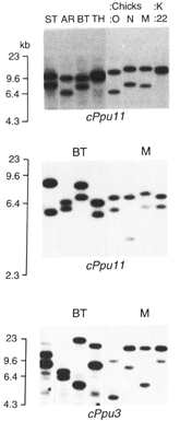
David Lank (1995) and his colleagues
used molecular probes called "mini-satellites" to determine which male sired
the chicks on ruff breeding grounds in Finland. By comparing the alleles in
chicks and alleles in the mother and putative sires, they were able to determine
the father and reconstruct the father's morphology (Fig. 2.1). They also scored
the morphology of the female parent's brother and father to determine the likely
phenotype that the female would have expressed had she been male. Such genetic
sleuthing is particularly important with sexually dimorphic traits which have
a sex-limited expression (e.g., traits only seen in males or only seen in females).
Females do not express the alternative male morphology, yet they might carry
genes for the morphology that they pass on to their male offspring. Lank and
his colleagues then reared the field caught chicks to maturity when they could
score the breeding morphology of the male progeny. They also reared an additional
generation of chicks in captivity that were derived from the field collected
cohort of chicks. They were certain of the father's identity in captive bred
birds and did not need to use molecular probes to determine paternity.

® Figure 2.2. Variation
in minisatellite alleles in male ruffs (ST, AR, BT, TH) that are used to determine
the sire of progeny (0, N, M) of the female (K:22). Allelic variation at three
microsatellite loci are shown (cPpu11, cPpu11, cPpu3). Given the mothers known
contribution to offspring, male BT is the only male that could be could contribute
alleles at all three loci and he is the likely sire.
Because only two phenotypes
are seen in the ruff, a single genetic locus with two alleles must be controlled
by a completely dominant allele and a recessive allele, otherwise we would expect
to see three phenotypes. The data on ruff pedigrees can discriminate between
several simple mendelian patterns of inheritance. Mendelian genes are either
found on sex chromosome or on autosomal chromosomes. Their genetic crosses rule
out the possibility that the gene is a sex-linked dominant (see below). Their
pedigree data is consistent with an autosomal gene with Satellite dominant.
While the example of male ruffs
provides solid evidence of major genes which affect the phenotype, the sample
size in these studies is still inadequate to test for the existence of other
genetic loci that control development of male behaviors. Testing for the effects
of two or more factors requires sample sizes in the thousands, particularly
if those factors interact epistatically or in a non-additive fashion.
Epistatic
Genes for Alternative Male Strategy and Sex Transformation in Marine Isopods
A final example of genes that
have a major effect on behavior involves the genetic control of alternative
male behaviors in a marine isopod, Paracerceis sculpta. Stephen Shuster
and his colleagues have characterized three alternative male morphs in the marine
isopod (Shuster and Wade, 1992, Shuster and Sassaman, 1997):
- a large alpha male with elongate
posterior appendages that they use to defend harems of females
- a medium-sized beta male that
can invade female harems by mimicking female behavior and morphology, and
- a small-sized gamma male that
invades female harems by virtue of its secretive behaviors.
In a large breeding study, based
on hundreds of genetic crosses, Shuster has developed a genetic model that explains
patterns of inheritance of the three morphs. Three alleles (a , b , g ) at the
Alternative male strategy (Ams) locus provide a reasonable explanation
of the general pattern of inheritance of the male morph. The three alleles have
the following dominance relations:
- b is dominant to both g and a
,
- g is dominant to a ,
- a is of course recessive to both
b and g .
The
a allele occurs at a very high frequency in the population (93%) compared to
either b (1%) or g (6%). An alpha male phenotype must be homozygous (e.g, a
|a ) at the Ams locus because a is recessive to the other to Ams
alleles. Gamma males can be either a |a or g |g . However, the heterozygous
form of gamma g |a is very common while the g |g form is rare in a natural populations.
Likewise, beta males can be b |g , b |a , or b |b . However, as a is the most
common allele in the population, the b |a is the most common genotype for a
beta male. As an exercise, compute the frequency of each male genotype assuming
Hardy-Weinberg gene frequencies and convince yourself that a |a , b |a , and
g |a are the most common male genotypes in the isopod population.
Shuster and Sassaman (1977)
found that a careful inspection of genetic crosses between females and the predominant
male genotypes revealed a significant departure from a 50:50 sex ratio of the
progeny. The existence of a second locus termed transformer (Tfr-two alternative
alleles, 1 and 2) is required to adequately explain the aberrant sex ratio
found only in certain genetic crosses. The Tfr locus causes males to
transform into females, or females to transform into males.
However, the direction of sex
change depends on the genotype at the Ams locus. Homozygous alpha males transform
from male to female if they bear at least one copy of the Tfr - 2 allele
(e.g., genotypes 1|2 and 2|2). Alpha males with the 1|1 genotype at the Tfr
locus are not sex-transformed. Conversely, beta males transform from female
to male if they bear at least one copy of the Tfr - 1 allele (e.g., genotypes
1|1 and 1|2). Beta males with the 2|2 genotype at the Tfr locus are not
sex-transformed. Gamma males transform from female to male if they are homozygous
for the Tfr-1 allele, but not if they carry one or more copies of the Tfr-2
allele. The epistatic interaction between two loci governs the expression of
male and female behaviors in this marine isopod. The gene for Alternative
male strategy interacts in a very non-additive fashion with the gene for
Transformer.
Finally, we find an added complexity
in this interesting genetic system. An extrachromosomal factor (ECF) accentuates
the effect of the Tfr locus, but only in the Tfr heterozygotes
of alpha and beta males. The exact nature of the ECF remains obscure but cytoplasmic
effects on that determine phenotype are common in the animal kingdom. They could
be transmitted from mother to egg (as are many cell organelles such as mitochondria).
Table 2.2. The interaction
between three alleles at the Alternative male strategy locus (Ams) and
two alleles at the Transformer locus (Tfr) in a marine isopod, Paracerceis
sculpta. See text for the dominance relations at the Ams locus. A plus symbol
with arrow (+) indicates a sex transformation owing to the alleles at the Tfr
locus. Alpha males that bear one or more copies of the Tfr-2 allele are
transformed into females during embryogenesis (pink). Conversely, Beta males
that bear a one or two copies of the Tfr-1 allele are transformed from
male to female (blue). The action of the Tfr gene can be accentuated
by the presence of an extrachromasomal factor ECF (* in blue). However, gamma
males are only transformed from female to male if they are homozygous for the
Tfr allele.
|
|
|
Tfr genotype
|
|
Ams genotype
|
SEX
|
1 1
|
1 2
|
2
2
|
|
a
a
|
M
F
|
-
-
|
-
ß *
+
|
-
ß
+
|
|
b
a
|
M
F
|
-
›
+
|
-
› *
+
|
-
-
|
|
g
a
|
M
F
|
-
›
+
|
-
-
|
-
-
|
Needless to say, analysis of
the genetic control of behaviors becomes a daunting task for anything but the
simplest genetic systems. As the number of genetic loci increases beyond three
or four it becomes increasingly difficult to isolate the expression of a phenotypic
trait to specific genes by using standard genetic crosses. The sample sizes
required become far to large in practice. Consider two loci each of which has
two alleles (A,a and B,b). Let us assume that alleles at both loci additively
act in the following fashion. Whereas the allele a adds nothing to phenotype,
the alternative allele A increments the phenotype by one unit. Likewise,
allele b adds nothing to phenotype, the alternative allele B increments
the phenotype by one unit. A Punnet square which describes the union of all
possible gametic types yields 16 genotye combinations and five phenotype combinations
(see Table 2.3).
Table 2.3. Punnett Square
for the effect of two loci which have purely additive effects.
|
|
AB
|
Ab
|
aB
|
ab
|
|
AB
|
AABB = 4
|
AABb = 3
|
AaBB = 3
|
AaBb = 2
|
|
Ab
|
AABb = 3
|
AAbb = 2
|
AaBb = 2
|
Aabb = 1
|
|
aB
|
AaBB = 3
|
AaBb = 2
|
aaBB = 2
|
aaBb = 1
|
|
ab
|
AaBb = 2
|
Aabb = 1
|
aaBb = 1
|
aabb = 0
|

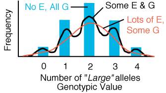
Figure 2.2.
Phenotype distribution of a trait governed by two mendelian loci that act additively
to produce the phenotype. If the phenotype is not affected by environmental
factors then 5 distinct modes are present. As phenotype becomes more and more
affected by random environmental factors, the phenotype distribution becomes
more and more normally distributed.
Rather than isolate the action
of single genes, quantitative genetic analyses assume that traits are due to
many genes of small effect, each of which act additively to produce the phenotype.
As the number of mendelian factors increase, and as more of the phenotype is
determined by environment, the distribution of many traits resembles a normal
distribution. The inheritance pattern of such polygenic traits is succinctly
described by a simple parameter known as heritability. The heritability reflects
the proportion of a phenotypic trait that is due to the additive genetic effect
of loci. The most straightforward way to estimate the heritability of a trait
is to measure the resemblance or correlation between relatives such as parents
and offspring, or between sibs.
A
major caveat of the quantitative genetic approach to behavioral genetics is
that it is quite difficult to build in epistatic effects such as those that
are seen in alternative male morphs of isopods. This is because additive effects
are easy to model. In contrast, epistatic models can take hundreds of possible
combinations for even a simple two or three locus system.
Side
Box 2.5: Heritability

A central aspect of Darwin's theory
of evolution includes a key statement: natural selection acts on traits that
are heritably transmitted between parents and offspring.
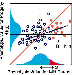
Darwin's cousin, Sir Francis Galton
coined the term for regression based on the observation that the regression
line which predicts offspring phenotype from a parent's phenotype always has
a slope less than one. The slope of the parent-offspring regression line is
also known as heritability. The heritability for any phenotypic trait
describes the proportion of the offspring's phenotype that we can predict from
a knowledge of the phenotype of both parents. The prediction is not exact and
includes some error about the regression line because offspring phenotype includes
environmental effects in addition to polygenic factors inherited from parents.
Finally, another formulation of heritability is derived from Eqn. 2.1:
heritability = h2 = G / P = G / (G + E).
Heritability is the proportion of
phenotypic variation (P = G + E) that is due to genetic causes (G). Because
phenotypic variation is larger than genetic variation, heritability be less
than one.
<END SIDE BOX>
It is possible for measured
heritability to be confounded with environment (Falconer, 1981). For example,
if parents and offspring share a common environmental factor which makes them
more similar by upbringing than genes alone heritability could be inflated.
In principle, a regression based upon any related individuals can be used to
estimate heritability. Sibs share the additive effects of alleles, much like
parents resemble offspring because of the additive effect of alleles. We could
use a correlation between sibs to predict h2, however, sibs have
an even greater tendency to share common environmental factors owing to their
common rearing environment, and h2 derived from
sibs is likely to be inflated owing to shared environment. Sibs not only share
additive effects of alleles, a common environment, but they also share another
component of variation referred to as dominance variation that makes them resemble
each other more so than they do their own parents.
Heritability
of IQ
Few arguments in behavior and
genetics are as contentious as those that rely on heritability estimates for
IQ. Periodically, a popular book arises that argues for genetically based differences
among racial or ethnic groups. These arguments invariably rely on estimates
of the heritability of IQ derived from twin studies. In a sense, it is perplexing
that something as well studied as IQ can remain so fiercely debated. For example,
in a recent study Devlin et al (1997) amassed 212 separate analyses of familial
resemblance which comprised 50,740 distinct pairings of varying degrees of relations.
Estimates of heritability were derived from the correlation between: mono-zygotic
twins, fraternal twins, siblings, parent and offspring, adoptive parents and
offspring.
If IQ were determined by a large
number of purely additive genes and did not include environmental influences,
then the coefficient of relatedness could be used to predict IQ. Because twins
share identical genes, a correlation between their IQ's should be close to the
theoretical maximum of 1.0 which assumes no environmental influences on IQ,
only additive genetic influences. The correlation for identical twins reared
together is 0.85, which suggests that at least part of IQ is environmental in
origin due to the common household. Perhaps, a better estimate for IQ would
be provided by using the IQ of 0.75 for twins that were "separated-at-birth"
and reared in different household environments. This still suggest a very strong
genetic component to intelligence as indexed by IQ tests.
However, the heritability estimate
based on twins still confounds a number of genetic and environmental factors.
Many popular arguments that rely on twin studies do not isolate the portion
of the correlation between relatives that is crucial to evolutionary arguments
-- the additive genetic variation. Another component of genetic variation that
is found between sibs does not contribute to evolutionary change -- dominance
variation. This dominance component is often inappropriately included in the
estimate of the heritability of IQ.
In order to clarify these issues,
Devlin et al (1997) used a technique called meta-analysis in which results from
a large number of individual studies of familial resemblance were used to estimate
various genetic and environmental influences on IQ. The model which best fit
the data included an additive genetic factor, a factor for dominance variation,
a factor for rearing household, and factor for pre-separation environment. The
pre-separation environment, which has been neglected in previous twin studies,
includes the common womb environment that twins would simultaneously share prior
to separation by adoption at or shortly after birth. Devlin et al (1997) found
that 20% of the variation in IQ was explained by a common womb environment.
While non-twin siblings share the same womb, they do not share it at the same
time, but sequentially share the womb. Only 5% of the overall resemblance in
IQ between ordinary siblings could be linked to this interesting maternal factor.
Devlin et al's study shows that variation in IQ has more to do with development
in the womb than previously thought. They suggest that many environmental agents
are likely causes of this environmental effect. For example, nutritional state,
smoking, and alcohol consumption by the pregnant mother are all known to lower
IQ.
From their results (1997) it
is clear that previous estimates based on twins have greatly overestimated the
heritability of IQ (e.g., as high as 60-80%). The heritability estimate which
excludes the confounding factors of maternal womb environment and common household
environment is on the order of 0.48. Finally, many IQ studies do not make an
important distinction between the total genetic variance in IQ and the additive
genetic variance. Any estimate of IQ from siblings confounds the additive genetic
component of IQ with the genetic component in IQ that arises from dominance
variation. All full siblings are expected to resemble one another a little more
than other family members owing to the possibility that they inherit a similar
dominance configuration from their parents (see side box on dominance). While
full siblings share this additional genetic source of resemblance, it is not
transmitted between parent and offspring. Thus, dominance variation is not an
important source of genetic variation underlying evolutionary change in intelligence.
The amount of additive genetic variation for IQ is estimated at 0.34 (excluding
dominance variation), which is still substantial but far lower than the amounts
generally purported for this interesting human behavior trait. Moreover, the
identified environmental factors such as the womb environment (5-20%), and the
common household environment (17%) total 22-37%, nearly the same as additive
genetic factors. Needless to say, improvement in human IQ could be brought about
by pre-natal and post-natal intervention.
Table 2.3. Correlations for
IQ among various degrees of familial resemblance (table modified from Devlin
et al, 1997). Note* : While the coefficient of relatedness is 0.5 for each parent,
if IQ were entirely due to additive genetic factors we could exactly predict
IQ of offspring from parents so we have the following total quantity of information
0.5 + 0.5 = 1.0 (Li, 1965).
|
Category of Familial Resemblance
|
Coefficient of Relatedness
|
Weighted Average Correlation
|
Why estimates for being reared together and apart differ.
|
Identical twins reared together
|
1.00
|
0.85
|
The common rearing environment of each twin leads to resemblance in IQ
that is not genetic.
|
Identical twins reared apart
|
1.00
|
0.74
|
The environment is more different than the environment of twins reared
together and who share a common household. Identical twins still share
a common womb environment.
|
Fraternal twins reared together
|
0.50
|
0.59
|
Fraternal twins share a common womb environment which might inflate their
resemblance. They are also reared together in the same place.
|
Siblings reared together
|
0.50
|
0.46
|
There are some environmental differences in the rearing environments.
|
Siblings reared apart
|
0.50
|
0.24
|
Common environmental differences in the rearing environments are eliminated,
but they still share common womb as do all sibs.
|
Mid-parent and child reared together
|
1.0*
|
0.50
|
The rearing environment that parents received from their own parents
might be expected to be preserved and transmitted to their own children.
However, the rearing environment could also be vastly different between
generations.
|
Single-parent and child reared together
|
0.50
|
0.41
|
This estimate is lower than that obtained for both parents , because
a single parent is a less accurate predictor of a child's genetic background.
However, this correlation still includes the possibility of common household
environment in upbringing of parents and offspring.
|
Single-parent and child reared apart
|
0.50
|
0.24
|
This correlation eliminates a common household environment in upbringing
of parents and offspring.
|
Adopting Parent and child
|
0.00
|
0.20
|
Resemblance must be largely due a common household environment in upbringing
of parents and offspring. Pure cultural transmission of IQ.
|
Relatives vary in the proportion
of alleles that they share in common, and the coefficient of relatedness is
a measure of the probability that an allele is in common between relatives.
For example, the coefficient of relatedness is 0.5 for one parent and offspring,
0.5 for sibs, 0.25 for half sibs, and 1.0 for dizygotic twins. By sharing alleles,
relatives end up sharing the additive effects of individual alleles.
While the relationship for the proportion of shared alleles between a parent
and an offspring is exact, the relationship between sibs is probabilistic. Offspring
get exactly one half of their genes from a single parent. However, it is theoretically
possible that full sibs could share none of their alleles, one of each pair
of alleles, or both pairs of the alleles (Li, 1965). How could this be? First
we can label alleles that parents could potentially give to their children:
1, 2 from their mother and 3, 4 from their father. Likewise, the situation where
sibs share no genes occurs with probability one-quarter for any given gene.
The most likely situation is when sibs share a single allele of a pair of alleles,
which occurs with probability of one-half. Finally, if offspring happen to share
both copies of their alleles in common they also share any dominance relations
between the two pairs of alleles that they inherit. This occurs with probability
one quarter for any given gene.
If sibs happen to share both
pairs of alleles 1 and 4, and 1 happens to be dominant to 4, then the sibs still
inherit the additive effect of the genes as well as the dominance variation.
Sibs still resemble each other largely because they share the additive effects
of genes. However, sharing a similar dominance configuration also increases
the resemblance between sibs relative to the resemblance between parents and
offspring. Sibs resemble each other more so than they do their parents. This
additional genetic component of variance is why some sibs appear to be identical
twins. The additional dominance variation that sibs share (no other relationship
shares this dominance variation) is also shared by twins. While full sibs share
dominance variation, offspring do not share dominance variation with their parents,
only additive genetic variance.
<END SIDE BOX>
We will end our discussion of
genetics on the importance of environmental factors. Up to this point in our
consideration of the genetic causes of behavior, we have treated the environment
as if it were some random factor that obscures the genetic transmission of behavior.
However, the environment can interact with genetic causes in interesting ways.
In particular, the genotype can be relatively fixed (e.g., little variation
among individuals), but the genetic machinery of development can still allow
the phenotype to develop into alternative types. We have already seen how genetic
differences among individuals can lead to alternative male phenotypes in marine
isopods and the ruffed grouse. The environment per se can also trigger alternative
developmental pathways that transform a juvenile into different morphologies
which have alternative behaviors (Smith-Gill 1983).
Condition-dependent
strategies and alternative male types
Many alternative male types
are thought to be condition-dependent strategies in which an organism's
internal physiological (e.g., nutrition, age, or body size) interacts with environmental
factors (e.g., food availability, hatching date, etc.) to alter development
of morphology and behavioral. Differences in morphology and behavior are not
governed by genetic factors such as alternative alleles. Blue-gill sunfish have
three alternative male phenotypes, however, the attempt to isolate alternative
alleles that control such behaviors have not been successful (Gross, 1984; Gross,
1991). It is thought that when males mature into three different-sized male
types with different behaviors, the trigger for the three states, is the overall
body-size at maturation. Males in good condition may mature later, and grow
into a large territorial male, that defends a small area in which females deposit
their eggs. The male is also parental and takes care of the brood. Males that
somewhat smaller, mature earlier, and develop into a female mimic that attempts
to fertilize the females eggs as the female attempts to oviposit them on a territorial
holding males nest. Finally, the smallest male type is thought to mature rapidly,
and at very small size. This sneaker male darts into a breeding pairs mating
ritual, and relies on confusion to obtain close access to the female and squirt
sperm on the run. Evidence that these types are environmentally determined is
provided by experimental manipulations of the availability of nest sites. If
nesting sites are restricted, the frequency of medium and small-sized males
increase, and the frequency of large parental males decreases (Gross, 1991)
<Drawing of Alternative Male
Strategies from M. Gross, see lecture>
Condition-dependent strategies
are also referred to as phenotypic plasticity. The phenotype of constant genotypes
are responding plastically to the environment. While the alternative phenotypes
are not controlled by alternative alleles, the development of the phenotype
is still governed by a cascade of events that are under some kind of genetic
control. The distinction is important because presumably all individuals in
a population are capable of developing into the alternative phenotypes, if their
environment had been conducive to these alternative developmental pathways from
the outset.
Alternative
Larval Types in Spadefoot Toads and Tiger Salamanders
A clear example of alternative
behaviors is seen in the development of larval amphibians. The interaction between
environment and the behaviors governing energy acquisition are central to the
growth and development of individuals. A basic dichotomy in feeding strategies
entails the distinction between carnivory and omnivory. Carnivores largely feed
on animals while ominvores tend to have a more catholic diet consisting of animals,
plants, and in some cases decaying plant and animal remains or detritus.
If you were to wander into the
deserts of the southwest during dusk after the hot July day has been chilled
by a torrential thunderstorm, you will find a small toad calling for mates.
Clustered around ephemeral pools filled with water, choruses of singing male
spadefoot toads try to attract females that are hopping towards the water to
lay their eggs. Water is a scarce resource for the toads and they emerge with
the first moistening of soil. Successful adult males clasp the back legs of
females in a tight amplectic embrace to stimulate the female to oviposit their
eggs. Fertilized eggs are left behind in the pool to develop. As you might have
already guessed, water does not last long in the glare of the summer desert
sun. Tadpoles that hatch from egg masses must develop rapidly into the terrestrial
adult form if they are to survive.
<Drawing of spadefoot toad lifecycle
from Pfennig, see lecture>
If a tadpole, happens to hatch
in a pond that is rich in a key resource, the fairy shrimp (a.k.a, Artemia
salina or sea monkeys), the tadpole might ingest enough shrimp and its development
can be profoundly altered (Pfennig 1990, 1990a). Tadpoles that eat a lot of
the shrimp are triggered to develop into a carnivore with specialized keratinized
tooth and large jaw musculature that is efficient for feeding on more shrimp.
Carnivores patrol the pond in a solitary fashion searching for their next meal.
If however, the tadpoles lands in a pool with few or no shrimp they develop
into an omnivore with a rasping jaw structure, a huge gut that allows for efficient
digestion of plant remains. Omnivores tend to swim in schools and the schooling
behaviors is thought to allow the group to stir up food more efficiently. Individuals
are capable of either the carnivorous or omnivorous morphology and behavior.
They only need to ingest enough shrimp to develop into the carnivorous form.
<picture of carnivore and omnivores
from Pfennig, see lecture>
What is the key environmental
factor in the shrimp? Shrimp are naturally loaded with the potent hormone thyroxine
and shrimp also have a heavy does of iodine a key component of thyroxine (Pfennig
1992b). Thyroxine is a key metabolic hormone found in all vertebrates, and also
governs development of juvenile amphibians, and controls the metamorphosis from
tadpole larva to terrestrial adult. By ingesting large amounts of this hormone,
the tadpoles precociously develop structures that allow for a more carnivorous
lifestyle, structures that are incidentally more reminiscent of the adult form.
David Penning performed critical experiments to show that high levels of thyroxine
precociously triggers development of the carnivores.
Carnivores develop much more
rapidly than the omnivore and carnivores metamorphose into toadlets in a shorter
period of time. The omnivore must consume greater quantities of food to reach
the size and stage required for metamorphosis to a terrestrial toadlet that
can escape the desiccating pool. Carnivores have a tremendous time advantage
in small ephemeral pools. Omnivores take longer to develop, but the tend to
metamorphose at a slightly a larger size, and with greater fat reserves. Omnivores
are successful in less ephemeral ponds. Moreover, the fairy shrimp is much more
abundant in the smaller faster drying ponds. The plasticity in development of
behavior and morphology is adaptive in that a female can leave progeny in a
small fast-drying pond or a larger long-standing pond, and the tadpoles environment,
presence or absence of shrimp determines the offspring's development.
1. What
additional genetic factors increase the resemblance between sibs besides additive
genetic variation?
2. Describe
a mutation experiment that was used to isolate a gene. Why is it important
to show that mice defective in this gene can perform non-nurturing tasks like
maze running or olfaction tests? What kinds of effects
do these additional tests detect? Why are we interested in a lack of effect
of a gene on other traits?
3. Why are
heritability estimates for sibs raised in different households preferable to
sibs raised in the same household? What additional confounding factors does
this design not remove from the heritability estimates?
4. You overhear
someone in the coffee shop citing the following evidence regarding heritability
of IQ: "IQ must be very heritable, the correlation between fraternal twins reared
by the same family is 0.59." "Hah!" the other combatant exclaims, "The correlation
between an adopted child and their unrelated sib is 0.20."
5. Compare and contrast genetic
determination and condition-dependent determination
of as proximate causes of alternative male strategies.
